![]()
![]()
by
Wenton L. Davis
![]()
![]()
This page is a quick tutorial on how to use SPICE circuit simulation tools. There are a LOT of versions of SPICE; most major manufacturers have their own variation of SPICE, and of course, they add their own particular idioms to their versions. I guess that's fair, if they are going to foot the bill for that much software, they should be allowed to do whatever ELSE they want, as long as the basics remain the same. That has had an interesting effect, though.... to my knowledge, there is absolutely no program that runs just plain, true, SPICE. Everything is "our version" of SPICE. (shrug) Just remember to always look up the user manual (or whatever documentation) for whichever specific version of SPICE you are using. Most of the examples on this page are using GNUcap. Well, OK, fine.... so here we go....
Many modern distributions of SPICE include several other components. SPICE, itself, is completely text-based. This would be mentally taxing for many modern computer users who are limited to only working in GUI environments. I strongly encourage people to learn to function in command-line environments, but as the years pass by, I find more and more that my encouragement falls on deaf ears. It therefore doesn't surprise me that most modern SPICE packages actually include GUI front-ends to handle drawing circuits (called "schematic capture") and for displaying the output in a prettier graphic output. I'll come back to the graphical display part, later. For this particular case, I want to focus strictly on working with SPICE as a text-mode only program because even in those larger packages, it is almost always possible to access the SPICE program from the command line, given enough user-friendly information.
![]()
![]()
![]()
Before going too far, I want to add a few links that can be used for reference. These links will describe some of the various cards to use in a SPICE program. NOTE: we use the term "card" in place of "line" because SPICE dates all the way back to the days of punchcards, and each command was listed on it's own card.
| components | controls | analysis |
And then, there's this one that really doesn't fit any real category:
![]()
![]()
![]()
To learn how to deal with a text-based description of a
circuit, take a look at the following circuit:
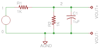
This circuit is a fairly simple one to study, but notice that there are several "nodes" that have been identified. Each circuit element must be described by where each component is connected, and these nodes are used to define these connections. Nodes can have any number, although it is almost universally standard to start at node 1 and count up. There is a node 0, which is ground. Some spice programs will allow you to use any node number as ground; some require that you use 0 as ground. SPICE will handle either situation. Any connection point (any point where any part of a component is connected to anything) must have a unique node number associated with it!
Once the nodes are defined in the circuit, it is time to define the circuit. In the previous example, using node 0 as ground, THe input voltage source, "Vin," is connected between nodes 0 and 1, so we define this in SPICE's language:
Vin 0 1 AC 1
which defines an independant voltage source, whose negative power is applied to ground and positive power is applied to node number 1. In this case, because we are going to do a frequency analysis, it is being defined as an AC voltage source with a peak voltage of 1V. We can continue to define the circuit with each of the elements:
  Vin 0 1 AC 1
  R1  1 2 1K
  R2  0 2 1K
  C1  0 2 1UF
Now that the circuit has been defined, it is important to put the details into the circuit file that will tell SPICE what to do with the circuit. One of the easiest parts to overlook is the title. Sure the title is just for decoration, but in this case, it could be meaning ful to include SOMETHING here, because if the title is ignored, SPICE will still give the circuit a title, which will be the first line of the file. So, include a .TITLE command as the first line of your file, and you'll be much happier with the results. The next, but arguably most important, thing to put into your circuit file, COMMENTS!!!!! Put comments in your file for many reasons, but most importantly, to describe what you are trying to accomplish! Comments in SPICE are any line beginning with an asterisk ('*') character. Although not required, I always (if I don't forget it) add a line to limit the width of text from my output with the command,
.OPTION OUT=80
which will tell SPICE to limit the width out output text to 80 characters. You can set it to more, but 80-120 seems to be a good balance, and anyone using Windoze will have tourble dealing with widths greater than 80. (Everybody write Bill Gates to complain!)
Finally, we need a few lines to tell SPICE how to perform it's analysis. Most versions of SPICE require that an " Operational Point" analysis must be done on the circuit before any of the other analysis are performed.
.PRINT OP V(2)
It doesn't really matter which node is selected (do NOT use node 0, which is ground; nothing ends up being analyzed), so I generally select my output node, which is node 2 in this case. Without it, the analysis will either not work at all, or it will probably be incorrect. I have seen a few circuits work without it, but only very simple DC Steady-state analysis seems to work without this.
Next, we need to define how to display the output. We could either print the output as a column of text, or we could create a graph of the output using text-graphing. admittedly, this is not as precise as GUI-based graphs, but we could take the column output and put it into a graphing program with almost no effort, and create some very nice graphs. (From here, it might be worth looking at another program called GNUplot, but I'll skip this for now.) To see a simple graph of the AC analysis of the output voltage (node 2), as a Bode plot between -20dB and 0dB, we can use the command:
.PLOT AC VDB(2)(-20,0)
Keep in mind that this line, itself, does NOT produce the analysis or the output. It simply tells SPICE that we are interested in a decibel (dB) plot of the output at node 2, within the scope of -20dB to 0dB. To actually perform the analysis and output, we will use the command:
.AC 5 1K OCT
This tells SPICE (finally) to perform the AC analysis using a series of frequencies, beginning a 5Hz, going up in octaves (an octave will be double the frequency, so in this case, the first octave will be 5Hz, ending when we have passed 1KHz, using one output per octave.
Our final circuit file looks like this:
  .TITLE Demonstration Circuit #1

  *Written by Wenton L. Davis, January 22, 2007
  *This is a simple circuit demonstration, showing some of the
  *basic structure for a simple AC circuit analysis.

  *============================================================
  * Define the circuit.  This is a simple R/RC voltage divider.
  *============================================================

  Vin 0 1 AC 1
  R1  1 2 1K
  R2  0 2 1K
  C1  0 2 1UF

  *============================================================
  * Define the output.
  *============================================================

  .OPTION OUT=80
  .PRINT OP V(2)

  .PLOT AC  VDB(2)(-20,0)

  *============================================================
  * Perform the analysis and output.
  *============================================================

  .AC 5 1K OCT
All that's left, now is to run the SPICE program and observe the output. To run the GNUcap program, the user just needs to type in the command:
~> gnucap -b demo1.ckt
This command tells GNUcap to run the circuit analysis program in batch mode (without user interaction) on the file, demo1.ckt. The output (using GNUcap) should look like this:
  Gnucap 2009.12.07 RCS 26.136
  The Gnu Circuit Analysis Package
  Never trust any version less than 1.0
  Copyright 1982-2002, Albert Davis
  Gnucap comes with ABSOLUTELY NO WARRANTY
  This is free software, and you are welcome
  to redistribute it under certain conditions
  according to the GNU General Public License.
  See the file "COPYING" for details.
  .TITLE Demonstration Circuit #1
  VDB(2)-20.              -15.             -10.              -5.               0.
          +-----------------+----------------+-----------------+----------------+
   5.     |                 .                .             *   .                |
   10.    |                 .                .             *   .                |
   20.    |                 .                .             *   .                |
   40.    |                 .                .             *   .                |
   80.    |                 .                .            *    .                |
   160.   |                 .                .          *      .                |
   320.   |                 .                .  *              .                |
   640.   |                 .     *          .                 .                |
   1.28K  |     *           .                .                 .                |
          +-----------------+----------------+-----------------+----------------+
In the output, it is easy to see that at low frequencies, the output is at -6dB, but at around 160Hz, the output starts to decrease, and beyond that, the output drops off fairly quickly.
![]()
![]()
![]()
Here is another example:
SPICE works based on a line-by-line description of the circuit, relating each component to a line in the program. It generally makes one assumption, that "GROUND" is node number 0. (This is not always true; some SPICE programs do not make this assumption... check the manufacturers' documentation!) Most discrete components (resistors, inductors, capacitors, power supplies, input signals) are one-line entries. A 1µF capacitor connected between nodes 2 and 5 named C3 is described in spice:
C3 2 5 1uFNow, if you haven't noticed, SPICE requires you to identify all of the nodes in the circuit. A node can be considered to be any point that multiple components are connected together. Even if a wire is seen on the schematic that travels a long distance, it is still considered to be the same node at both ends (unless you are trying to model that long wire with inductance, stray capacitance, and inherent resistance).
So, let's consider a very simple example. In
circuit 1, a small signal is applied to a simple low-pass filter.
Ground is assumed to be node 0, the input is applied to node 1, the resistor
and capacitor meet at node 2, which is also the output, and the capacitor is
also connected to ground.
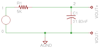
Which would be translated into SPICE:
.TITLE One Pole

VIN 1 0 AC 1 SIN(0 1 1KHz)
R1  1 2 5K
C1  2 3 31.83E-09
Now a few things to point out; VIN is an AC signal source, the DC offset is 0, the amplitude is 1V, and the frequency is 1KHz. SPICE will also accept 31.83E-09, 31.83n to mean the same value, and it will assume you mean Farads, with or without the "F" on the end. How else are you going to measure capacitance? (I have to be careful - I had one student get mad at me because I would not give her a "straight" answer to, "how many Amps in a Volt?") As will be apparent, later, this notation is important when coupling to other programs. For now, let's just be happy that SPICE will accept whatever format we give it.
From here, I find it convenient ("necessary") to provide an output with. SPICE will gladly assume your terminal window is 80 characters wide. ICK! Because it is so easy (in linux) to widen the window, I issue the command:
.OPTION OUT=150to inform SPICE that it can produce output as wide as 150 characters.
And now for something I don't understand, but it makes things work: include the line:
.PRINT OP V(2)(change V(2) to whichever node you want for your output). I have no idea what this does, but things fail to work if this does not exist.
Now, the outputs can be defined. Here, the first output is a transient analysis, observing V(1) and V(2), the voltages at nodes 1 and 2, assuming each is in the range -3<V<3:
.PLOT TRAN V(1) (-3,3) V(2) (-3,3)and the second output is a frequency analysis (over-riding the 1KHz defeinition), ranging from 10Hz to 10MHz on a decade (logarithmic) scale with 10 steps per decade, observing the range from -55dB to +5dB:
.PLOT AC VDB(2) (-55,5)
The analysis is finally performed with the following lines:
.TRAN 0.01MS 1MS 0.05MS

.AC DEC 10 10 10Meg
NOTE the capitol "M" still referes to "milli-" and "Meg" refers to "mega-" as exponent modifiers! (This will cause probelms, I promise!) So, mush it all together to create the file:
.TITLE One Pole

VS 1 0 AC 1 SIN(0 1 1KHz)
R1 1 2 5K
C1 2 0 31.83E-09

.OPTION OUT=150

.PRINT OP V(2)
.PLOT TRAN V(1) (-3,3) V(2) (-3,3)
*.PRINT TRAN V(1) V(2)

.PLOT AC VDB(2) (-55,5)
*.PRINT AC VDB(2)

.TRAN 0.01Ms 1MS 0.05MS

.AC DEC 10 10 10MEG

.END
To run the simulation, you have the choice of running in "batch" mode (run and exit), or in "interactive" mode (read file and accept input from the terminal). As should be obvious by now, I do not claim to be any kind of SPICE expert, just trying to provide useful tips. So, I will only say - I have not mastered the interactive mode and if you want to try it on your own..... go for it! Otherwise, I generally run in batch mode. Assuming that the file above was saved in the file, onepole.ckt, type the command:
>gnucap -b onepole.cktfrom which I get the output:
Gnucap 2009.12.07 RCS 26.136
The Gnu Circuit Analysis Package
Never trust any version less than 1.0
Copyright 1982-2006, Albert Davis
Gnucap comes with ABSOLUTELY NO WARRANTY
This is free software, and you are welcome
to redistribute it under certain conditions
according to the GNU General Public License.
See the file "COPYING" for details.
.TITLE One Pole
V(1) -3. -1.5 0. 1.5 3.
V(2) -3. -1.5 0. 1.5 3.
+----------------------------------+----------------------------------+----------------------------------+----------------------------------+
50.u | . .+ * . |
60.u | . .+ * . |
70.u | . . + * . |
80.u | . . + * . |
90.u | . . + * . |
100.u | . . + * . |
110.u | . . + * . |
120.u | . . + * . |
130.u | . . + * . |
140.u | . . + * . |
150.u | . . + * . |
160.u | . . + * . |
170.u | . . + * . |
180.u | . . + * . |
190.u | . . + * . |
200.u | . . + * . |
210.u | . . + * . |
220.u | . . + * . |
230.u | . . + * . |
240.u | . . + * . |
250.u | . . + * . |
260.u | . . + * . |
270.u | . . + * . |
280.u | . . + * . |
290.u | . . + * . |
300.u | . . + * . |
310.u | . . + * . |
320.u | . . + * . |
330.u | . . + * . |
340.u | . . + * . |
350.u | . . +* . |
360.u | . . * . |
370.u | . . *+ . |
380.u | . . * + . |
390.u | . . * + . |
400.u | . . * + . |
410.u | . . * + . |
420.u | . . * + . |
430.u | . . * + . |
440.u | . . * + . |
450.u | . . * + . |
460.u | . . * + . |
470.u | . . * + . |
480.u | . . * + . |
490.u | . .* + . |
500.u | . * + . |
510.u | . *. + . |
520.u | . * . + . |
530.u | . * . + . |
540.u | . * . + . |
550.u | . * . + . |
560.u | . * . + . |
570.u | . * . + . |
580.u | . * . + . |
590.u | . * . + . |
600.u | . * . + . |
610.u | . * . + . |
620.u | . * .+ . |
630.u | . * + . |
640.u | . * +. . |
650.u | . * + . . |
660.u | . * + . . |
670.u | . * + . . |
680.u | . * + . . |
690.u | . * + . . |
700.u | . * + . . |
710.u | . * + . . |
720.u | . * + . . |
730.u | . * + . . |
740.u | . * + . . |
750.u | . * + . . |
760.u | . * + . . |
770.u | . * + . . |
780.u | . * + . . |
790.u | . * + . . |
800.u | . * + . . |
810.u | . * + . . |
820.u | . * + . . |
830.u | . * + . . |
840.u | . * + . . |
850.u | . * + . . |
860.u | . * + . . |
870.u | . *+ . . |
880.u | . * . . |
890.u | . +* . . |
900.u | . + * . . |
910.u | . + * . . |
920.u | . + * . . |
930.u | . + * . . |
940.u | . + * . . |
950.u | . + * . . |
960.u | . + * . . |
970.u | . + * . . |
980.u | . + * . . |
990.u | . + *. . |
0.001 | . + * . |
+----------------------------------+----------------------------------+----------------------------------+----------------------------------+
VDB(2)-55. -40. -25. -10. 5.
+----------------------------------+----------------------------------+----------------------------------+----------------------------------+
10. | . . . * |
12.589 | . . . * |
15.849 | . . . * |
19.953 | . . . * |
25.119 | . . . * |
31.623 | . . . * |
39.811 | . . . * |
50.119 | . . . * |
63.096 | . . . * |
79.433 | . . . * |
100. | . . . * |
125.89 | . . . * |
158.49 | . . . * |
199.53 | . . . * |
251.19 | . . . * |
316.23 | . . . * |
398.11 | . . . * |
501.19 | . . . * |
630.96 | . . . * |
794.33 | . . . * |
1.K | . . . * |
1.2589K| . . . * |
1.5849K| . . . * |
1.9953K| . . . * |
2.5119K| . . . * |
3.1623K| . . *. |
3.9811K| . . * . |
5.0119K| . . * . |
6.3096K| . . * . |
7.9433K| . . * . |
10.K | . . * . |
12.589K| . . * . |
15.849K| . . * . |
19.953K| . * . . |
25.119K| . * . . |
31.623K| . * . . |
39.811K| . * . . |
50.119K| . * . . |
63.096K| . * . . |
79.433K| . * . . |
100.K | * . . |
125.89K| * . . . |
158.49K| * . . . |
199.53K| * . . . |
251.19K| * . . . |
316.23K| * . . . |
398.11K| * . . . |
501.19K| * . . . |
630.96K* . . . |
794.33K* . . . |
1.Meg * . . . |
1.2589M* . . . |
1.5849M* . . . |
1.9953M* . . . |
2.5119M* . . . |
3.1623M* . . . |
3.9811M* . . . |
5.0119M* . . . |
6.3096M* . . . |
7.9433M* . . . |
10.Meg * . . . |
+----------------------------------+----------------------------------+----------------------------------+----------------------------------+
NOTE: Web browsers may or may not like this. If your web broswer line-wrapped, sorry. Such is the result if you use OUTPUT=150 and only have an 80-column window. There are alternatives....
Yes, it is "plotted" in text mode. Guess what - this is how SPICE looks! Oh, I hear it now... "I can't use this; it's icky!" Yes, it is. So, go back to the file and change the two .PLOT commands to .PRINT, delete the ranges (-3,3) and (-55,5) and re-run. Now, you get:
Gnucap 2009.12.07 RCS 26.136
The Gnu Circuit Analysis Package
Never trust any version less than 1.0
Copyright 1982-2006, Albert Davis
Gnucap comes with ABSOLUTELY NO WARRANTY
This is free software, and you are welcome
to redistribute it under certain conditions
according to the GNU General Public License.
See the file "COPYING" for details.
.TITLE One Pole
#Time       V(1)       V(2)
 50.u       0.30902    0.044171
 60.u       0.36812    0.062105
 70.u       0.42578    0.082504
 80.u       0.48175    0.10512
 90.u       0.53583    0.12971
 100.u      0.58779    0.15604
 110.u      0.63742    0.18385
 120.u      0.68455    0.21292
 130.u      0.72897    0.243
 140.u      0.77051    0.27387
 150.u      0.80902    0.3053
 160.u      0.84433    0.33706
 170.u      0.87631    0.36894
 180.u      0.90483    0.40072
 190.u      0.92978    0.43219
 200.u      0.95106    0.46315
 210.u      0.96858    0.49341
 220.u      0.98229    0.52277
 230.u      0.99211    0.55106
 240.u      0.99803    0.57811
 250.u      1.         0.60375
 260.u      0.99803    0.62783
 270.u      0.99211    0.6502
 280.u      0.98229    0.67073
 290.u      0.96858    0.6893
 300.u      0.95106    0.70578
 310.u      0.92978    0.72007
 320.u      0.90483    0.73209
 330.u      0.87631    0.74174
 340.u      0.84433    0.74896
 350.u      0.80902    0.7537
 360.u      0.77051    0.7559
 370.u      0.72897    0.75552
 380.u      0.68455    0.75255
 390.u      0.63742    0.74697
 400.u      0.58779    0.73879
 410.u      0.53583    0.728
 420.u      0.48175    0.71465
 430.u      0.42578    0.69876
 440.u      0.36812    0.68037
 450.u      0.30902    0.65955
 460.u      0.24869    0.63636
 470.u      0.18738    0.61087
 480.u      0.12533    0.58318
 490.u      0.062791   0.55339
 500.u      1.0432n    0.52159
 510.u     -0.062791   0.4879
 520.u     -0.12533    0.45245
 530.u     -0.18738    0.41536
 540.u     -0.24869    0.37677
 550.u     -0.30902    0.33683
 560.u     -0.36812    0.29569
 570.u     -0.42578    0.25349
 580.u     -0.48175    0.2104
 590.u     -0.53583    0.16659
 600.u     -0.58779    0.12222
 610.u     -0.63742    0.077452
 620.u     -0.68455    0.032466
 630.u     -0.72897   -0.012567
 640.u     -0.77051   -0.057476
 650.u     -0.80902   -0.10209
 660.u     -0.84433   -0.14623
 670.u     -0.87631   -0.18973
 680.u     -0.90483   -0.23243
 690.u     -0.92978   -0.27415
 700.u     -0.95106   -0.31474
 710.u     -0.96858   -0.35404
 720.u     -0.98229   -0.39189
 730.u     -0.99211   -0.42816
 740.u     -0.99803   -0.46269
 750.u     -1.        -0.49537
 760.u     -0.99803   -0.52605
 770.u     -0.99211   -0.55462
 780.u     -0.98229   -0.58097
 790.u     -0.96858   -0.605
 800.u     -0.95106   -0.62662
 810.u     -0.92978   -0.64574
 820.u     -0.90483   -0.66228
 830.u     -0.87631   -0.67619
 840.u     -0.84433   -0.6874
 850.u     -0.80902   -0.69589
 860.u     -0.77051   -0.70161
 870.u     -0.72897   -0.70454
 880.u     -0.68455   -0.70467
 890.u     -0.63742   -0.70201
 900.u     -0.58779   -0.69657
 910.u     -0.53583   -0.68836
 920.u     -0.48175   -0.67742
 930.u     -0.42578   -0.66379
 940.u     -0.36812   -0.64754
 950.u     -0.30902   -0.62871
 960.u     -0.24869   -0.6074
 970.u     -0.18738   -0.58368
 980.u     -0.12533   -0.55765
 990.u     -0.062791  -0.52941
 0.001     -998.14p   -0.49907
#Freq       VDB(2)
 10.       -434.25u
 12.589    -688.21u
 15.849    -0.0010907
 19.953    -0.0017285
 25.119    -0.0027392
 31.623    -0.0043405
 39.811    -0.0068772
 50.119    -0.010895
 63.096    -0.017254
 79.433    -0.027314
 100.      -0.043211
 125.89    -0.068287
 158.49    -0.10774
 199.53    -0.16953
 251.19    -0.26571
 316.23    -0.4139
 398.11    -0.63888
 501.19    -0.97317
 630.96    -1.4553
 794.33    -2.1243
 1.K       -3.0102
 1.2589K   -4.1243
 1.5849K   -5.4552
 1.9953K   -6.973
 2.5119K   -8.6387
 3.1623K   -10.414
 3.9811K   -12.265
 5.0119K   -14.169
 6.3096K   -16.107
 7.9433K   -18.068
 10.K      -20.043
 12.589K   -22.027
 15.849K   -24.017
 19.953K   -26.011
 25.119K   -28.007
 31.623K   -30.004
 39.811K   -32.002
 50.119K   -34.001
 63.096K   -36.001
 79.433K   -38.
 100.K     -40.
 125.89K   -42.
 158.49K   -44.
 199.53K   -46.
 251.19K   -48.
 316.23K   -50.
 398.11K   -52.
 501.19K   -54.
 630.96K   -56.
 794.33K   -58.
 1.Meg     -60.
 1.2589Meg -62.
 1.5849Meg -64.
 1.9953Meg -66.
 2.5119Meg -68.
 3.1623Meg -70.
 3.9811Meg -72.
 5.0119Meg -74.
 6.3096Meg -76.
 7.9433Meg -78.
 10.Meg    -80.
"This isn't much better!" Well.... maybe it is. For the non-unicians out there, let me just point out that unix (and various flavors) is arguably the most ecclectic set of tools ever assembled! This output can be saved to a file, and with a little massaging, it can be fed into gnuplot. This is discussed on my GNUcap and GNUplot page. GNUplot has been ported to Windoze as well, so Windoze users aren't without all hope.
One important note before continuing... the .PLOT command will, at MOST, display two plots at the same time. of more value, the .PRINT command will output many columns of data, where the first column is always the X-axis, and subsequent columns are Y-values at that location on the X-axis. Again, this is great for use with GNUcap and GNUplot!
![]()
![]()
![]()
An example of a transistor circuit: note that the
transistor is REALLY distorting:
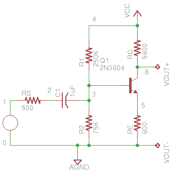
Here is the circuit description:
.TITLE NPN Distortion

VCC 4 0 5

VS 1 0 AC 1 SIN(0 1 1KHz)
RS 1 2 500
C1 2 3 1u
R1 3 4 250K
R2 3 0 75K
RC 5 4 5600
RE 6 0 600

Q1 5 3 6 Q2N3904

.MODEL Q2N3904 NPN BF=120 IS=1.E-12

.OPTION OUT=150

.PRINT OP V(5)
*.PLOT TRAN V(5) (0,5) V(6) (-0,5)
.PRINT TRAN V(5) V(6)

.TRAN 0.0S 2MS 0.00001S

*.AC DEC 10 10 10MEG

.END
And here is an over-simplified Op-amp example:
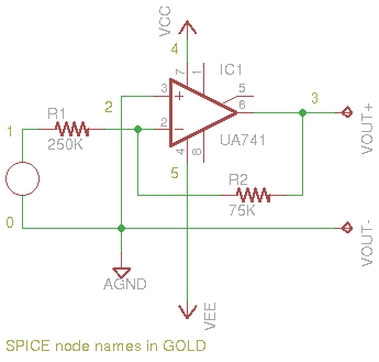
And its description:
.TITLE OP-amp Example

VCC 4 0 20
VEE 5 0 -20

VS 1 0 AC 1 SIN(0 1 10KHz)
R1 1 2 5K
R2 2 3 10K
XOP1 0 2 0 4 5 3 UA741


.SUBCKT OPAMP1 1 2 6
RIN 1 2 10MEG
EP1 3 0 1 2 100K
RP1 3 4 1K
CP1 4 0 1.5915UF

EOUT 5 0 4 0 1
ROUT 5 6 1
.ENDS


.SUBCKT UA741    1   2   3   4    5    6
*               Vi+ Vi- GND PWR+ PWR- Vout
Q1 11 1 13 OPNPN1
Q2 12 2 14 OPNPN2
RC1 4 11 5.305165E+03
RC2 4 12 5.305165E+03
C1 11 12 5.459553E-12
RE1 13 10 2.151297E+03
RE2 14 10 2.151297E+03
IEE 10 5 1.666000E-05
CE  10 3 3.000000E-12
RE  10 3 1.200480E+07
GCM 3 21 10 3 5.960753E-09
GA 21 3 12 11 1.884955E-04
R2 21 3 1.000000E+05
C2 21 22 3.000000E-11
GB 22 3 21 3 2.357851E+02
RO2 22 3 4.500000E+01
D1 22 31 OPD12
D2 31 22 OPD12
EC 31 3 6 3 1.0
RO1 22 6 3.000000E+01
D3 6 24 OPD34
VC 4 24 2.803238E+00
D4 25 6 OPD34
VE 25 5 2.803238E+00
.MODEL OPD12 D (IS=9.762287E-11)
.MODEL OPD34 D (IS=8.000000E-16)
.MODEL OPNPN1 NPN (IS=8.000000E-16 BF=9.166667E+01)
.MODEL OPNPN2 NPN( IS=8.309478E-16 BF=1.178571E+02)
.ENDS

.OPTION OUT=150

.PRINT OP V(3)
*.PLOT TRAN V(1) (-3,3) V(3) (-3,3)
.PRINT TRAN V(1) V(3)

*.PLOT AC VDB(3) (-5,15)
.PRINT AC VDB(3)

*.PLOT AC VDB(3) (-5,15)
.PRINT AC VDB(3)

.TRAN 0.01Ms 0.2MS 0.005MS

.AC DEC 10 10 10MEG

.END
![]()
![]()
![]()
Now that we can get the output, let's go back and look at that header:
Gnucap 2009.12.07 RCS 26.136
The Gnu Circuit Analysis Package
Never trust any version less than 1.0
Copyright 1982-2006, Albert Davis
Gnucap comes with ABSOLUTELY NO WARRANTY
This is free software, and you are welcome
to redistribute it under certain conditions
according to the GNU General Public License.
See the file "COPYING" for details.
.TITLE Lab 5
#Time       V(1)       V(2)       V(3)
50.u       0.80902    0.4542     0.46065
51.u       0.74174    0.42064    0.42672
52.u       0.66601    0.38249    0.38824
53.u       0.58269    0.34017    0.34563
etc...
OK, Dr. Davis, thank you for providing gnucap, and for warning us that it is not a completed project. Now, MAKE THAT MESSAGE GO AWAY!!! No, OK, fine, we'll do it ourselves. We can just use the tail command:
gnucap -b lab5.ckt | tail -n +10
This will throw away the first 9 lines, and continue the text output, beginning with the 10th line.
Next, we might want to translate the Meg, M (milli), u, n, p, and f to their appropriate x10n values. We can use the "stream editor," sed, to search for each of these:
gnucap -b lab5.ckt | tail -n +10 | sed s/Meg/E+06/g | sed s/K/E+03/g | sed s/M/E-03/g | sed s/u/E-06/g | sed s/n/E-09/g | sed s/p/E-12/g | sed s/f/E-15
Yes, it's a lot of typing; either deal with it, or write a script to perform the filtering. But this is still important because we can direct the output to a file, using the `> filename` to save the filtered results to a file. If, for example, you save the output to something called "lab5.out" then you can use gnuplot to plot the output in a much nicer output than the .PLOT command in gnucap will show:
gnuplot> plot 'lab5.out' using 1:4 with lines
will open the file, 'lab5.out' and use column 1 as the X-axis coordinate value and column 4 as the Y-axis coordinate value, and connect the dots with lines. (The default is to use '+' symbols.)
Now that you are all edumicatified in SPICE, you can try it out for yourself! Just go here to try it online!
![]()
![]()
![]()